TrueVisualization & clustering of embeddings
Visualization of embeddings
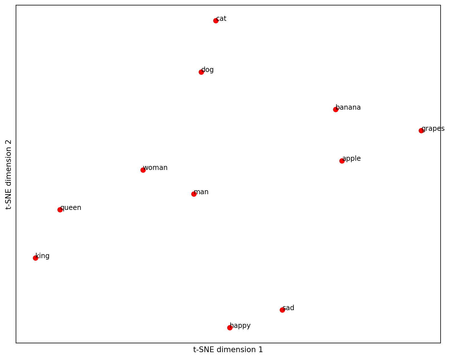
Let’s go a little bit further down the road of similarities between words or texts in general. Wouldn’t it be great if we could somehow visualize a text as a point in space and see how other texts relate to it? Embeddings allow us to do that as well, with one caveat: Embeddings have too many dimensions to visualize (usually a few thousand). Luckily, there are tools such as principal component analysis or T-SNE available to reduce the dimension of vectors (for example, to two dimensions), while preserving most of the relations between them. Let’s see how this works.
# prerequisites
import os
from openai import OpenAI

MODEL = "text-embedding-3-small" # choose the embedding model

# get the OpenAI client
client = OpenAI(
    api_key=os.environ.get("OPENAI_API_KEY")
)
# Define a list of words to visualize
words = ["king", "queen", "man", "woman", "apple", "banana", "grapes", "cat", "dog", "happy", "sad"]
# Get embeddings for the words
response = client.embeddings.create(
input=words,
model=MODEL
)
embeddings = [emb.embedding for emb in response.data]import numpy as np
import matplotlib.pyplot as plt
from sklearn.manifold import TSNE
# Apply t-SNE dimensionality reduction
tsne = TSNE(
n_components=2,
random_state=42,
perplexity=5 # see documentation to set this correctly
)
embeddings_2d = tsne.fit_transform(np.array(embeddings))
# Plot the embeddings in a two-dimensional scatter plot
plt.figure(figsize=(10, 8))
for i, word in enumerate(words):
x, y = embeddings_2d[i]
plt.scatter(x, y, marker='o', color='red')
plt.text(x, y, word, fontsize=9)
plt.xlabel("t-SNE dimension 1")
plt.ylabel("t-SNE dimension 2")
plt.grid(True)
plt.xticks([])
plt.yticks([])
plt.show()
Clustering of embeddings
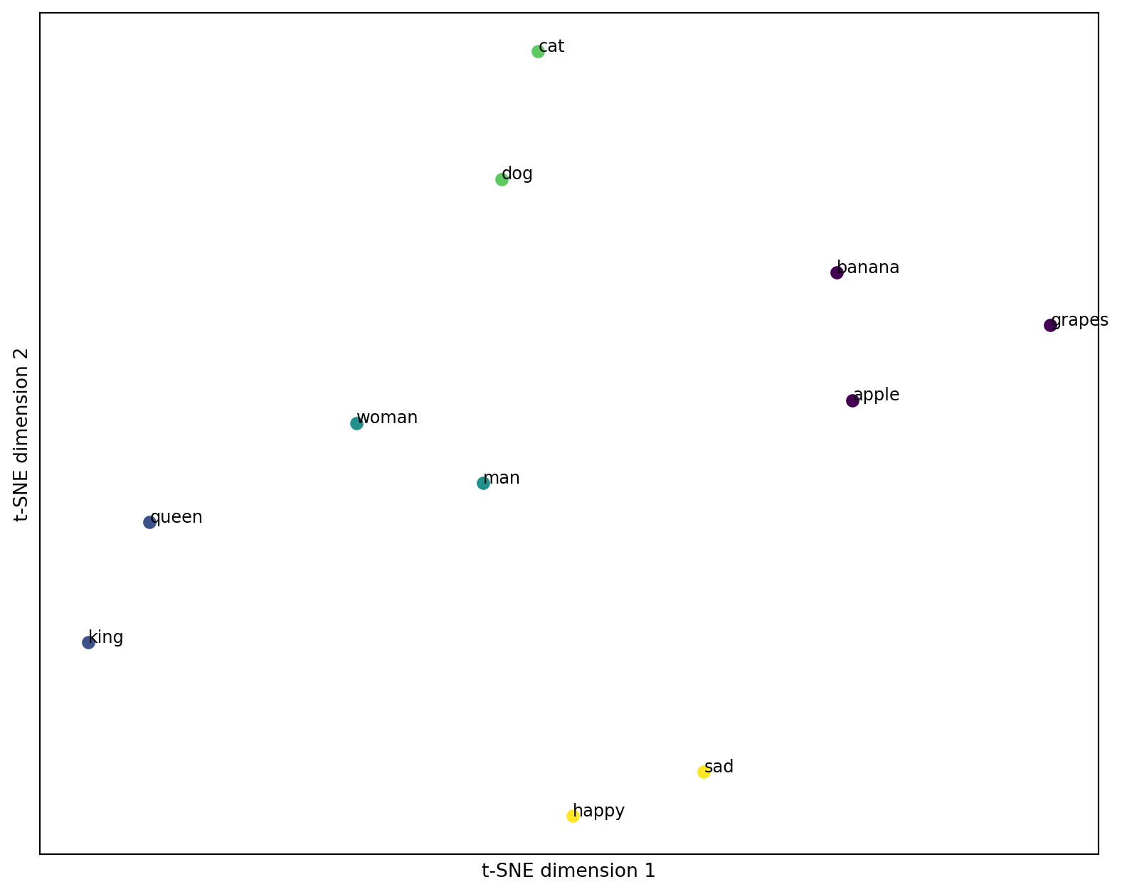
The great thing is, we can already see that there are some clusters forming. We can again use models like KMeans to find them explicitly. In this case, we obviously have five clusters, so let’s try to identify them.
# do the clustering
import numpy as np
from sklearn.cluster import KMeans

n_clusters = 5

# define the model
kmeans = KMeans(
  n_clusters=n_clusters,
  n_init="auto",
  random_state=2 # do this to get the same output
)

# fit the model to the data
kmeans.fit(np.array(embeddings))

# get the cluster labels
cluster_labels = kmeans.labels_
import matplotlib.pyplot as plt
from sklearn.manifold import TSNE
# Apply t-SNE dimensionality reduction
tsne = TSNE(
n_components=2,
random_state=42,
perplexity=5 # see documentation to set this correctly
)
embeddings_2d = tsne.fit_transform(np.array(embeddings))
# Define a color map for clusters
colors = plt.cm.viridis(np.linspace(0, 1, n_clusters))
# Plot the embeddings in a two-dimensional scatter plot
plt.figure(figsize=(10, 8))
for i, word in enumerate(words):
x, y = embeddings_2d[i]
cluster_label = cluster_labels[i]
color = colors[cluster_label]
plt.scatter(x, y, marker='o', color=color)
plt.text(x, y, word, fontsize=9)
plt.xlabel("t-SNE dimension 1")
plt.ylabel("t-SNE dimension 2")
plt.grid(True)
plt.xticks([])
plt.yticks([])
plt.show()
That, again, is great news. Embeddings allow us to find clusters in texts, based on the semantics included. This helps in many applications where documents need to be analyzed without having been seen by a human. Maybe you can use it in your project?